Category: mathematics

  • propagation of errors: Arithmetic errors

    propagation of errors: Arithmetic errors

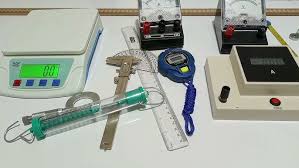
    Propagation of errors is when error is accounted for in arithmetic error operations with the measured values. The measured values are being used for addition, subtraction, multiplication and division along with their errors.

    What do we do with errors when we have found them?

    propagation of errors in Addition and subtraction

    Addition and subtraction is when we account for errors while summing up values that have errors. we discuss this with an example:

    consider the rectangle with lengths 14.75 cm, 8.96, cm, 14.75 cm, 8.96 cm as shown.

    A rectangle measured with propagation of errors

    suppose we need to find it’s perimeter. To achieve that, we are to add the lengths of each side. we have the following measurements:

    The errors in measurement of length = (1/2) x 0.01 = 0.005 cm

    The errors in measurement of width= (1/2) x 0.01 = 0.005 cm

    maximum possible length = 14.755 cm

    minimum possible length = 14.745 cm

    maximum possible width = 8.965 cm

    minimum possible width = 8.955 cm

    because we have upper and lower limits of lengths then we have 3 possible sums that gives the perimeter:

    • when we use the upper limits in measured lengths to find perimeter
    • when we use the lower limits in measured lengths to find perimeter
    • perimeter when we use the actual measured values without errors.

    maximum possible perimeter =14.755 cm + 14.755 cm + 8.965 cm +8.965 cm = 47.44 cm

    minimum possible perimeter = 14. 745 cm + 14. 745 cm + 8.955 cm + 8.955 cm = 47.40 cm

    working perimeter = 14.75 cm + 14.75 cm + 8.96 cm + 8.96 cm =47.42 cm

    absolute error in sum = maximum sum – working sum

    That is : | 47.44 – 47.42 | = 0.02

    similarly; absolute error = | working sum – minimum sum | =| 47.42 – 47.40 | = 0.02

    $$\text{relative error in perimeter} = \frac{0.02}{47.42} = 0.000422 $$
    Example in propagation of errors

    Calculate error in 1.23 m – 0.67 m

    solution

    $$ \text{The measurements lie within } 1.23 \pm 0.005 \text{ and } 0.67 \pm 0.005 $$

    The maximum possible difference will be obtained when we subtract the minimum value of subtrahend from maximum of the minuend.

    that is, maximum difference = 1.235 – 0.665 = 0.57

    The minimum possible difference is when we subtract the the maximum value of subtrahend from minimum of the minuend.

    that is; minimum =1.225 – 0.675 = 0.55

    the working difference = 1.23 – 0.67 = 0.56

    absolute error = | 0.56 – 0.55| or | 0.57 – 0.56 | = 0.01

    propagation of errors in Multiplication: product errors

    To calculate errors involving multiplication, we need to find working area, maximum possible area and the minimum possible area.

    consider our earlier rectangle which we redraw here:

    suppose we need to find it’s area.

    $$ \text{The measurements lie within } 14.75 \pm 0.005 \text{ and } 8.96 \pm 0.005 $$
    $$ \text{maximum possible error} = 14.755 \times 8.965 = 132.278575 $$
    $$ \text{minimum possible error} = 14.745 \times 8.955 = 132.041475 $$
    $$ \text{working area} = 14.75 \times 8.96 = 132.1600 $$

    The working area is NOT midway between the lower and the upper limits

    $$ \text{maximum area} – \text{working area} = 132.278575 – 132.1600 = 0.118575$$
    $$ \text{working area} – \text{minimum area}= 132.1600 – 132. 041475= 0.118525$$

    The absolute error in products is the average of the two differences above expressed as:

    $$\text{absolute error in area} = \frac{0.118575 + 0.118525}{2} = 0.11855$$

    the absolute error in area can also be calculated from average difference between the maximum area and minimum area

    that is :

    $$\text{absolute error in area} = \frac{1}{2}{\text{maximum area}-\text{minimum area}}$$

    in our example: we have

    $$\text{absolute error in area} = \frac{1}{2}({132.278575}-{132.041475}) =\frac{1}{2} \times 0.2371 = 0.11855$$

    calculating relative error in the area

    $$\text{relative error in area} = \frac{\text{absolute error in area}}{\text{working area}} $$

    in our case:

    $$\text{relative error in area} = \frac{0.11855}{132.1600} = 0.000897 $$

    Alternative procedure of calculating relative error in area

    relative error in product can also be calculated from relative errors of the individual measurements. Relative error can also be expressed as the sum of the relative errors in individual measurements.

    for example considering our triangle.

    $$\text{relative error in length} = \frac{0.005}{14.75} = 0.000339$$
    $$\text{relative error in width} = \frac{0.005}{8.96} =0.000558$$
    $$\text{relative error in area } = ( 0.000339 + 0.000558) = 0.000897$$

    Error in quotient (Division error)

    While working on relative error in division, we calculate largest possible quotient, smallest possible quotient and the working quotient.

    consider finding density of substance given it’s mass as 5.79 g and it’s volume as 4.63 cm3 .

    $$Density (\rho) = \frac{mass}{volume} $$
    $$Density (\rho) = \frac{5.79}{4.63} = 1.25054$$

    The maximum possible quotient will be given by the maximum possible value of the numerator and the smallest possible value of the denominator.

    $$ \text{maximum possible quotient} = \frac{\text{maximum numerator}}{\text{miminum numerator} }$$

    in our example:

    $$ \text{maximum possible quotient} = \frac{5.795}{4.625 } = 1.25297$$
    $$ \text{minimum possible quotient} = \frac{5.785}{4.635 } = 1.24811$$
    $$\text{absolute error in quotient} = \frac{1}{2} \times (\text{maximum possible quotient} – \text{minimum possible quotient})$$
    $$\text{absolute error in quotient} = \frac{1}{2} \times (1.25297 – 1.24811)=\frac{1}{2}\times 0.00486=0.00243$$

    Relative error in quotient

    $$\text{Relative error in quotient} = \frac{\text{absolute error in quotient}}{\text{working quotient}} $$

    in our example:

    $$\text{Relative error in quotient} = \frac{0.00243}{1.25054} = 0.00194 $$

    Related topics

  • Accuracy of measuring instruments

    Accuracy of measuring instruments

    There is always a small difference between a measured value and the actual value.

    This occurs regardless of the accuracy in the measuring instrument. Measured values are then said to be the approximations or estimates of the actual values.

    The difference between the actual value and the measured values is referred to as the error.

    Accuracy in measuring instruments

    Measuring instruments are usually calibrated with markings. There is always a gap between two marking. If the measured objects fall between the two calibrated markings, we must estimate. The reason is, we cannot read the actual value.

    Accuracy of a measuring instruments depends on the smallest units of measurements that is being used in the instrument. An ordinary ruler can measure lengths up to the nearest millimeter. This is because the smallest units of measurements used in a ruler is one millimeter.

    If a length is 5.5 cm, it means it is nearer 5.5 cm than any other value on the ruler. However, the measurements is said to lie on the neighborhoods of 5.5 cm. This neighborhood is 5.45 cm and 5.55 cm.

    5.45 cm is then said to be the lower limit while 5.55 cm is said to be the upper limit.

    For a micrometer screw gauge, the smallest unit of measurements is 0.01 mm or 0.001 cm. A measurements given in centimeters from micrometer screw gauge will thus have three decimal places. For example 5.892 cm. This means the measurements is between 5.8915 cm and 5.8925 cm.

    A micrometer screw gauge measures lengths to a higher degree of accuracy. This is due to the increased number of decimal places making it more precise compared to a ruler.

    Absolute error

    When a measuring instruments has the least units of measurements as 0.1 cm, measuring 7.5 cm causes the greatest possible error to be 7.55 cm -7.5 cm = 0.05 cm or 7.5 cm – 7.55 cm = -0.05 cm.

    We are only interested in the size of the possible error. Therefore, we ignore the sign. We state the absolute error as 0.05 cm. thus, |-0.05| = |+0.05| = 0.05

    in general, when the accuracy of the instrument is 0.1, the measured value n can be described as:

    $$n-0.05 \leq n \leq n+0.5 $$

    In other words, Absolute error is usually calculated as half of the smallest unit of measurements unless otherwise stated. For example if measurement is given as 7.612 cm, the smallest unit of measurements is 0.001 cm. the absolute error will thus be given as :

    $$\text{absolute error} = \frac{1}{2} \times \text{smallest unit of measurement}$$

    in this case, it should be:

    $$\text{absolute error} = \frac{1}{2} \times 0.001 = 0.0005$$

    Relative error

    Errors involved in measuring small quantities has more effects than errors in large quantities. For example, an error of 0.05 m when measuring a length that is not more than 2 m is significant. This error can be large compared to the same error while measuring a length of 200 km.

    Relative error is used to gauge error with respect to the measured value.

    $$\text{relative error} = \frac{\text{absolute error}}{\text{actual measurement}}$$

    For example, the relative error for measuring 2 m will be given by:

    $$\text{relative error} = \frac{0.05}{2.0} = 0.025$$

    The relative error when measuring 200 km would be :

    $$\text{relative error} = \frac{0.05}{200000.0} = 0.00000025$$

    The later error calculated is small enough and can be considered negligible compared to the size being measured.

    Percentage error

    percentage error is relative error expressed as percentage. That is;

    $$\text{percentage error} = \frac{\text{absolute error}}{\text{actual measurement}} \times 100$$

    in the case mentioned above, the first case will have percentage error given as:

    $$\text{percentage error} = \frac{0.05}{2.0} \times 100 = 2.5\%$$

    the second case will have the percentage error given by:

    $$\text{percentage error} = \frac{0.05}{200000.0} \times 100 = 0.000025 \%=$$

    Measurements with an error of 2.5% is less reliable compared to that with 0.000025%

    Practice exercise

    in each of the following, determine: upper limit, lower limit, absolute error, relative error and the percentage error:

    (a) 60.70 Kg (b) 2.5 m (c) 6.5 cm (d)800.9 m (e) 800 m (f)16.295 m

    Round off error

    It is the difference between the rounded value and the original value before round off.

    example if we round of 3.674 to two decimal places, we have round off error computed as follow:

    value after round off = 3.67

    3.674 – 3.67 = 0.004

    Truncating error

    Truncating is slashing off figures from numbers without rounding off:

    for example, 345.7867844 can be truncated to 2 decimal places to give 345.78. If it was round off, it should be 345.79

    Related topics


  • Integration by substitution

    Integration by substitution

    illustrating integration by substitution by replacing u for x-1

    Page Contents

    In Calculus, Integration by substitution is when we replace an integral value or its parts in an attempt to make the expression easier to integrate.

    Consider the function f(u) such that u is a function of x.

    let u = f(x) and f(u)=u

    ddxf(u)=dudxf′(u)ddxf(u)=dudxf′(u)

    where:

    f′(u)=df(u)duf′(u)=df(u)du

    Integrating….;

    ∫dudxf′(u)dx=∫ddxf(u)dx=f(u)+C∫dudxf′(u)dx=∫ddxf(u)dx=f(u)+C

    but:

    f′(u)=df(u)duf′(u)=df(u)du

    so that

    ∫f′(u)du=f(u)+c∫f′(u)du=f(u)+c

    ∫dudxf′(u)dx=∫f′(u)du=f(u)+C∫dudxf′(u)dx=∫f′(u)du=f(u)+C

    Example 1

    Solve the problem below using Integration by substitution:

    ∫x2√x3+5∫x2x3+5

    solution

    substitute the expression under the root sign as shown:

    let

    u=x3+5u=x3+5

    then integrating u with respect to x we get:

    dudx=3x2dudx=3×2

    and so:

    du=3x2dxdu=3x2dx

    and making dx the subject:

    dx=du3x2dx=du3x2

    rewriting the expression:

    ∫x2√x3+5=∫x2√udu3x2∫x2x3+5=∫x2udu3x2

    x2 on the numerator can then be cancelled out by the x2 on the denominator.

    The expression becomes:

    ∫√Udu3x2=∫u123du∫Udu3x2=∫u123du

    =

    =13∫U12du=13∫U12du

    13.U3232+C=2U329+C13.U3232+C=2U329+C

    13.U3232+C=2U329+C=29(x3+5)32+C13.U3232+C=2U329+C=29(x3+5)32+C


    Example 2

    solve :

    ∫2x√1+x2dx∫2×1+x2dx

    solution

    let u = 1 +x2

    then differentiating u with respect to x

    dudx=2ududx=2u

    and then rearranging:

    dx=du2xdx=du2x

    then rewriting the integral:

    ∫2x√udu2x=∫√udu∫2xudu2x=∫udu

    2x on the denominator has cancelled the 2x on the numerator so that we only have u that is easy to integrate:

    ∫√udu=∫u−12du=[u3232+C]∫udu=∫u−12du=[u3232+C]

    =2u323+C=2(1+x2)323+C=2u323+C=2(1+x2)323+C

    Example

    solve by substitution:

    ∫1√2x+1dx∫12x+1dx

    solution

    let u = 2x + 1

    differentiating u with respect to x we obtain;

    dudx=2dudx=2

    now we express dx in terms of u as:

    du=dx2du=dx2

    Then we need to rewrite our integral as:

    ∫1u12du2=12∫u−12du∫1u12du2=12∫u−12du

    then:

    ∫u−12du=12[u1212]+C∫u−12du=12[u1212]+C

    =U12+C=U12+C

    rem U = 2x + 1

    and any number raised to power of 1/2 is like finding it’s squareroot

    hence:

    U12+C=√2x+1+CU12+C=2x+1+C

    substitution Problem involving trigonometric ratios

    solve:

    ∫cosxsin3xdx∫cosxsin3xdx

    solution:

    let u = sin x: then

    dudx=cosxdudx=cosx

    dx=ducosxdx=ducosx

    and applying substitution in our integral, we replace dx;

    ∫cosxsin3xdx=∫cosx.u3ducosx∫cosxsin3xdx=∫cosx.u3ducosx

    cos x in the numerator cancels the one at the denominator that the expression is reduced to:

    ∫u3du∫u3du

    ∫u3du=U44+C∫u3du=U44+C

    but u = sin x; therefore:

    U44+C=sin4x4+CU44+C=sin4x4+C

    generally:

    ∫cosxsinxxdx=1n+1sinn+1+C∫cosxsinxxdx=1n+1sinn+1+C

    Example on trigonometric substitution

    solve:

    ∫sinxcos5xdx∫sinxcos5xdx

    solution

    let u = cos x

    du=−sinxdxdu=−sinxdx

    du−sinx=dxdu−sinx=dx

    rewriting dx in our original integral:

    ∫sinxcos5xdx=∫sinxcos5xdu−sinx∫sinxcos5xdx=∫sinxcos5xdu−sinx

    we eliminate sin x in the integral to obtain the following expression:

    =∫−cos5xdu=∫−cos5xdu

    but cos x = u

    hence cos5x = u5 and so the integral becomes:

    −∫u5du−∫u5du

    hence we get:

    −∫u5du=−u66+6−∫u5du=−u66+6

    and then replacing u for cos x we get:

    −cos6x6+C−cos6x6+C

    in general:

    ∫sinxcosnxdx=−1n+1cosn+1x+C∫sinxcosnxdx=−1n+1cosn+1x+C

    Integration by substitution: natural log by substitution

    solve:

    ∫lnxxdx∫lnxxdx

    solution

    let u = lnx

    dudx=1xdudx=1x

    x du = dx

    hence we write the integral as:

    ∫lnxxdx=∫lnxxxdu∫lnxxdx=∫lnxxxdu

    and so we eliminate x to have the integral:

    ∫lnxdu=∫udu∫lnxdu=∫udu

    ∫udu=u22+C=(lnx)22+C∫udu=u22+C=(lnx)22+C

    Example on sec trigonometric ration

    solve:

    ∫sec2(3x−1)dx∫sec2(3x−1)dx

    solution

    let u = 3x-1

    dudx=3dudx=3

    du = 3dx

    dx=du3dx=du3

    ∫sec2udu3=13∫sec2udu=13tanu+c=13tan(3x−1)+C∫sec2udu3=13∫sec2udu=13tanu+c=13tan(3x−1)+C

    Example 3 on trigonometric ratio

    integrate:

    ∫sinxecosxdx∫sinxecosxdx

    solution

    let u = cos x

    du=−sinxdxdu=−sinxdx

    dx=du−sinxdx=du−sinx

    =∫sinxeudu−sinx=−∫eudu=−eu+c=∫sinxeudu−sinx=−∫eudu=−eu+c

    Practice exercise

    use the substitution method to evaluate the following integrals:

    1.∫x(x2−3)4dx∫x(x2−3)4dx

    2.∫x√1−x2dx∫x1−x2dx

    3.∫cos2x(sin(2x+3))2dx∫cos2x(sin(2x+3))2dx

    4.∫ex√1+exdx∫ex1+exdx

    5.∫sec2xtan2xdx∫sec2xtan2xdx

    6.∫√x√1+x32dx∫x1+x32dx

    7.∫(x+1)sin(x2+2x+2)dx∫(x+1)sin(x2+2x+2)dx

    8.∫(x+1)√x2+2x+3dx∫(x+1)x2+2x+3dx

    9.∫x2(x3+8)4dx∫x2(x3+8)4dx

    Related Topics

  • The Electromagnetic spectrum: Frequency range and wavelengths

    The Electromagnetic spectrum: Frequency range and wavelengths

    The electromagnetic (EM) spectrum is the range of all types of Electromagnetic  radiation. Radiation is energy that travels and spreads out as it goes – the visible light that comes from a lamp in your house and the radio waves that come from a radio station are two types of electromagnetic radiation.

    Electromagnetic waves are transverse waves which results from oscillating electric and magnetic fields at right angles to each other.

    Electromagnetic spectra are arranged in order of their wavelength or frequency. This arrangement forms what is known as the electromagnetic spectrum.

    A complete spectrum is shown below:

    The figure below shows electromagnetic waves arranged in order of decreasing wavelengths

    Properties of Electromagnetic waves

    The Electromagnetic waves have the following common properties.

    • They travel through vacuum(space) with a speed of 3.0 x 10⁸ms-1 . This speed is usually referred to as the speed of light in vacuum and is usually denoted by c.
    • Do not require material medium for transmission
    • They are transverse in nature
    • Electromagnetic waves undergoes interference, reflection,refraction and polarisation effect
    • Posses energy in different amounts according to the relation E=hf where h is the Plank’s constant given as 6.63 x 10⁻³⁴ Js and f is the frequency
    • They carry no charge
    • They are not affected by electric or magnetic fields
    Example: calculating energy of a wave

    A certain electromagnetic radiation was found to be having a wavelength of 6.5 x 10⁻⁸ m. Calculate the energy it emits.

    solution

    To calculate the energy of a wave, you need to know its frequency. Then multiply the frequency by Planck’s constant.

    Here we have only the wavelength, but we can get the frequency from the relation: v = fλ.

    since it is an electromagnetic wave, it’s speed is 3.0 x 10⁻⁸ ms-1. and hence f=v/λ. that is:

    =4.6154 x 10¹⁵ HZ

    The energy of a wave was defined as E = hf where h (plank’s constant)= 6.63×10⁻³⁴ Js

    hence E = 6.63 x 10-34 Js x 4.6154 x 1015 HZ 3.06 x 10⁻²⁰J.

    Related Topics


    References

    • Secondary Physics Student’s Book Four. 3rd ed., Kenya Literature Bureau, 2012. pp.
    • Abbot A. F. (1980), Ordinary Level Physics, 3rd Edition, Heinemann Books International,
      London.
    • Nelkon M. and Parker P., (1987), Advanced Level Physics, Heinemann Educational Publishers, London.
    • Tom D., and Heather K. Cambridge IGCSE Physics. 3rd ed., Hodder Education, 2018, https://doi.org/978 1 4441 76421.